Introduction to R Programming

Learning objectives

understand the basics of R programming
Understand data types and objects
understand base (built-in) R functions

Reading

Basics of R

In the previous section, we showed the layout of RStudio. For this lesson, you will write all the code in the scripts/source and see the output in the console. To comment on the code, you will use the hashtag (#) to tell R not to execute the line as a code.

R can be used as a calculator:

4 + 7

[1] 11

9 * 6

[1] 54

Arithmetic Operators

Description	Operator	Example
Addition	+	1 + 3
Subtract	-	90 - 5
Multiplication	*	6 * 7
Exponentiation	^	3 ^ 6
Division	/	54 / 7

Type in and run the above examples in the script or console.

Assignment operator

Notice that we have been running previous codes without assigning them to objects. We use the assignment operator (<-) in R to assign whatever we have created into object; this can be a plot, a variable, a table, etc. Using above example, let us recreate our code but assigning them:

addition <- 4 + 7 

print(addition)

[1] 11

multiplication <- 9 * 6 

print(multiplication)

[1] 54

Notice in the above code, we have told R to create an object called ‘addition’ and every time we call print() function, the results will be printed in the console. Please remember the assignment operator (<-) as we will use it through this course. We can also assign objects using =:

addition = 4 + 7

print(addition)

[1] 11

However, many R programmers and I use the <- operator for a serious reasons; so we will stick to it.

Also, you do not necessarily need to call the print() function in order to print results/output, you can just write the name of the object you have created, run it and it will be printed:

river_km <- 1200

river_km

[1] 1200

Notice that the object river_km when we print the object river_km, it prints what is inside of it, the element on the console.

Basically, we have created variables (addition, multiplication, river_km). With these variables, we can perform basic analysis:

tugela_length <- 502

orange_river_length <- 2200

# Find the difference in river length
orange_river_length - tugela_length

[1] 1698

# sum of rivers

orange_river_length + tugela_length

[1] 2702

Data types in R

There 3 basic data types in R

character: strings, text, etc
numeric: numbers, can be integers or whole numbers
logical: TRUE/FALSE, also called Boolean

An example of a character:

river <- "Tugela"

province <- "KZN"

Notice that a character need to be surrounded by (““) every time, otherwise R will return an error

river <- Tugela

Error in eval(expr, envir, enclos): object 'Tugela' not found

province <- KZN

Error in eval(expr, envir, enclos): object 'KZN' not found

An example of a numerical:

tugela_length_km <- 502

orange_river_length <- 2200

numericals do not to need to be surrounded by " ", if you do, they will be stored as numeric.

An example of a logical data type:

kzn <- TRUE

kzn

[1] TRUE

gauteng <- FALSE

gauteng

[1] FALSE

You can ask R to tell you the type of the data structure by using class() function:

class(tugela_length_km)

[1] "numeric"

class(orange_river_length)

[1] "numeric"

class(river)

[1] "character"

class(gauteng)

[1] "logical"

Base R functions

R has built-in functions that we can use to analyse and manipulate data. A function is always followed by (). We will use examples to illustrate various R functions.

Summary statistics

Basic summary statistics functions are mean, median, range, standard deviation, etc. We can get in R using the mean() function:

# first create a vector of numbers ("numeric vector")

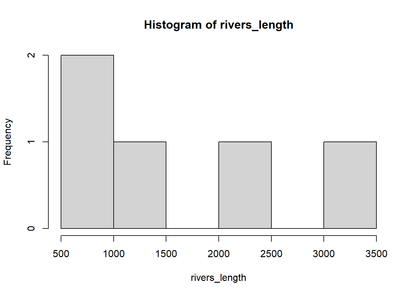
rivers_length <- c(502, 2200, 1500, 3050, 800)

rivers_length

[1]  502 2200 1500 3050  800

mean(rivers_length)

[1] 1610.4

The mean of a rivers_length variable we have created is 1610.4.

We can use the median() function to get the median of our variable:

median(rivers_length)

[1] 1500

The median age is 1500

And also the standard deviation using sd() function:

sd(rivers_length)

[1] 1038.937

You can get minimum and maximum values using min() and max() functions, respectively:

min(rivers_length)

[1] 502

max(rivers_length)

[1] 3050

You can create a basic plot using a hist() function:

hist(rivers_length)

You may want to arrange the values into ascending or descending order using the sort() function:

sort(rivers_length) # sort into ascending order

[1]  502  800 1500 2200 3050

sort(rivers_length, decreasing = T) # sort into descending order

[1] 3050 2200 1500  800  502

In this section, you have learnt basic data types, functions and operators. Next, we learn different type of data structures.