Dataframes, as we saw the previous section, is a tabular data format, with columns and rows. Columns are variable names and rows are individual observations.
Let us a basic data frame with three columns: country, life expectancy, and population of Southern African countries. First, we create individual vectors:
# Create a character vectorcountry_name <-c("Angola", "Botswana", "Lesotho", "Malawi", "Mozambique", "Namibia", "South Africa", "Swaziland", "Zambia", "Zimbabwe")country_name
Because we have 3 vectors of equal length, we can create a dataframe, using a data.frame() function:
southern_africa_df <-data.frame(country_name, life_expectancy, population) #combine two vectors to create a dataframesouthern_africa_df ## print the dataframe
A dataframe is basically made of vectors (columns). In the southern_africa_df dataframe, we have 3 columns: country_name, life_expectancypopulation. We can extract these elements using the $ sign:
We will use the dplyr package to manipulate data. dplyr is part of tidyverse meta-package and is mostly used to clean, manipulate and transform dataframes. dplyr has 5 main verbs/functions:
select(): for selecting particular columns in a dataframe
filter(): for sub-setting rows based on the specified criteria
arrange(): sort rows/observations based (ascending/descending)
summarise(): for summary statistics
mutate(): create new columns based on the manipulation of the existing columns.
group_by(): get aggregate statistics by a category
library(dplyr)
Attaching package: 'dplyr'
The following objects are masked from 'package:stats':

    filter, lag
The following objects are masked from 'package:base':

    intersect, setdiff, setequal, union
You can also load dplyr by loading the tidyverse package; this will load all the packages in in `tidyverse at once. This is useful, for example, when you want to clean and visualise data:
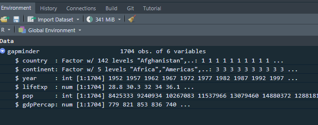
Now you have an object, which is a dataframe, called gapminder, you can see it in the Environment pane in RStudio. It shows that it has ncol(gapminder) columns/variables and nrow(gapminder) observations/rows
gapminder dataframe in Environment pane
You can use the str() fucntion to get the structure of the dataframe:
You can get a sample of the first observations/rows using head() function:
head(gapminder)
# A tibble: 6 × 6
  country     continent  year lifeExp      pop gdpPercap
  <chr>       <chr>     <int>   <dbl>    <int>     <dbl>
1 Afghanistan Asia       1952    28.8  8425333      779.
2 Afghanistan Asia       1957    30.3  9240934      821.
3 Afghanistan Asia       1962    32.0 10267083      853.
4 Afghanistan Asia       1967    34.0 11537966      836.
5 Afghanistan Asia       1972    36.1 13079460      740.
6 Afghanistan Asia       1977    38.4 14880372      786.
4.1.4 select() function
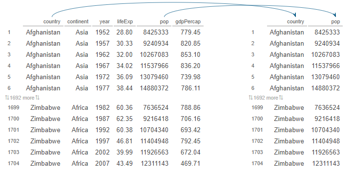
We may be interested in some of the columns in the gampminder dataframe, let say, for example, “country” and “pop” variables and discard others; we use the select() function:
Then using the select() function to select only pop and country columns
You will that pipe becomes important when having multiple chains of functions at once.
You will notice that in other sources: web, books, etc. have %>% instead of |>. It works the same way. The |> is new. %>% comes from mgttr, an external package, so you needed to load it first before using it. The native pipe |> is built in R, so it there is no need to load it. So, we will stick with the |>.
In your RStudio, follow these instructions:
Go to ‘Tools’ and click on ‘Global Options’
Navigate to ‘Code’ on the left pane
Then select the fourth option, “use native pipe operator, |>”
Click ‘Apply’
You can use the short cut Ctrl + Shift + M If you using Windows to insert the pipe instead of typing it. If you are using Mac, use Cmd + Shift + M.
4.1.4 Return to select() function
As I have said, select() only return the columns specified
Also, notice that we selected “country’ and”pop” columns but did not save them and assigned to an object. To store the results into an object, we have to use assignment operator (<-):
Now we have saved results as gapminder_selected, and we can do other analysis with this object because we have saved it. So, in a nutshell, when you run a code without assigning results into an object, using the <- operator, results will not be saved but will be printed.
You can also select columns based by index/position. Let us select only 1st and 3rd coulmns
# A tibble: 1,704 × 3
   country     continent  year
   <chr>       <chr>     <int>
 1 Afghanistan Asia       1952
 2 Afghanistan Asia       1957
 3 Afghanistan Asia       1962
 4 Afghanistan Asia       1967
 5 Afghanistan Asia       1972
 6 Afghanistan Asia       1977
 7 Afghanistan Asia       1982
 8 Afghanistan Asia       1987
 9 Afghanistan Asia       1992
10 Afghanistan Asia       1997
# ℹ 1,694 more rows
Here, we have select columns from country to year only.
You can also exclude certain columns by simply adding the minus (-) sign; let say we want to exclude the gdpPercap from the dataframe
gapminder |>select(-gdpPercap)
# A tibble: 1,704 × 5
   country     continent  year lifeExp      pop
   <chr>       <chr>     <int>   <dbl>    <int>
 1 Afghanistan Asia       1952    28.8  8425333
 2 Afghanistan Asia       1957    30.3  9240934
 3 Afghanistan Asia       1962    32.0 10267083
 4 Afghanistan Asia       1967    34.0 11537966
 5 Afghanistan Asia       1972    36.1 13079460
 6 Afghanistan Asia       1977    38.4 14880372
 7 Afghanistan Asia       1982    39.9 12881816
 8 Afghanistan Asia       1987    40.8 13867957
 9 Afghanistan Asia       1992    41.7 16317921
10 Afghanistan Asia       1997    41.8 22227415
# ℹ 1,694 more rows
4.1.5 filter() function
You may be interested in observations/rows that meet certain conditions. We use filter() function to return the list that meet our conditions. filter() has several operators:
==: equal to
!=: not equal to
>: greater than
<: less than
>=: greater than or equal to
<=: less than or equal to
Let us filter based on the continent column. How many continent are there? Create a basic table first
table(gapminder$continent)
  Africa Americas     Asia   Europe  Oceania
     624      300      396      360       24
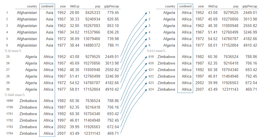
There are five continents. Let us filter only observations from the African continent:
# A tibble: 624 × 6
   country continent  year lifeExp      pop gdpPercap
   <chr>   <chr>     <int>   <dbl>    <int>     <dbl>
 1 Algeria Africa     1952    43.1  9279525     2449.
 2 Algeria Africa     1957    45.7 10270856     3014.
 3 Algeria Africa     1962    48.3 11000948     2551.
 4 Algeria Africa     1967    51.4 12760499     3247.
 5 Algeria Africa     1972    54.5 14760787     4183.
 6 Algeria Africa     1977    58.0 17152804     4910.
 7 Algeria Africa     1982    61.4 20033753     5745.
 8 Algeria Africa     1987    65.8 23254956     5681.
 9 Algeria Africa     1992    67.7 26298373     5023.
10 Algeria Africa     1997    69.2 29072015     4797.
# ℹ 614 more rows
africa_gapminder object is a dataframe we have just created, with only countries from the African continent. What filter() does is to return observations/rows that only meet our conditions:
Let us filter a numeric column; for example, we may want to filter countries with population of above 50 million and assign results to an object named high_pop:
# A tibble: 1,020 × 6
   country     continent  year lifeExp      pop gdpPercap
   <chr>       <chr>     <int>   <dbl>    <int>     <dbl>
 1 Afghanistan Asia       1952    28.8  8425333      779.
 2 Afghanistan Asia       1957    30.3  9240934      821.
 3 Afghanistan Asia       1962    32.0 10267083      853.
 4 Afghanistan Asia       1967    34.0 11537966      836.
 5 Afghanistan Asia       1972    36.1 13079460      740.
 6 Afghanistan Asia       1977    38.4 14880372      786.
 7 Afghanistan Asia       1982    39.9 12881816      978.
 8 Afghanistan Asia       1987    40.8 13867957      852.
 9 Afghanistan Asia       1992    41.7 16317921      649.
10 Afghanistan Asia       1997    41.8 22227415      635.
# ℹ 1,010 more rows
Sometimes you may need to filter multiple rows, let say, more than 5 countries. It would be inconvinient to type country == "..." five times. This is where the %in% operator is useful:
# A tibble: 5 × 6
  country      continent  year lifeExp      pop gdpPercap
  <chr>        <chr>     <int>   <dbl>    <int>     <dbl>
1 Ghana        Africa     2007    60.0 22873338     1328.
2 South Africa Africa     2007    49.3 43997828     9270.
3 Tanzania     Africa     2007    52.5 38139640     1107.
4 Tunisia      Africa     2007    73.9 10276158     7093.
5 Zimbabwe     Africa     2007    43.5 12311143      470.
4.1.6 arrange() function
arrange() function is self-explanatory: it sort values into ascending or descending order
africa_2007 |>arrange(lifeExp) |>head(n =10) ## show the first 10 observations
# A tibble: 10 × 6
   country                  continent  year lifeExp      pop gdpPercap
   <chr>                    <chr>     <int>   <dbl>    <int>     <dbl>
 1 Swaziland                Africa     2007    39.6  1133066     4513.
 2 Mozambique               Africa     2007    42.1 19951656      824.
 3 Zambia                   Africa     2007    42.4 11746035     1271.
 4 Sierra Leone             Africa     2007    42.6  6144562      863.
 5 Lesotho                  Africa     2007    42.6  2012649     1569.
 6 Angola                   Africa     2007    42.7 12420476     4797.
 7 Zimbabwe                 Africa     2007    43.5 12311143      470.
 8 Central African Republic Africa     2007    44.7  4369038      706.
 9 Liberia                  Africa     2007    45.7  3193942      415.
10 Rwanda                   Africa     2007    46.2  8860588      863.
The default sorting is ascending order; you can sort into descending order by using desc() function within arrange():
africa_2007 |>arrange(desc(lifeExp)) |>head(n =10) ## show the first 10 observations
# A tibble: 10 × 6
   country               continent  year lifeExp      pop gdpPercap
   <chr>                 <chr>     <int>   <dbl>    <int>     <dbl>
 1 Reunion               Africa     2007    76.4   798094     7670.
 2 Libya                 Africa     2007    74.0  6036914    12057.
 3 Tunisia               Africa     2007    73.9 10276158     7093.
 4 Mauritius             Africa     2007    72.8  1250882    10957.
 5 Algeria               Africa     2007    72.3 33333216     6223.
 6 Egypt                 Africa     2007    71.3 80264543     5581.
 7 Morocco               Africa     2007    71.2 33757175     3820.
 8 Sao Tome and Principe Africa     2007    65.5   199579     1598.
 9 Comoros               Africa     2007    65.2   710960      986.
10 Mauritania            Africa     2007    64.2  3270065     1803.
4.1.7 summarise()
We use the summarise() function to get the summary statistics. Common statistics include mean, median, standard deviation, minimum, maximum, etc.
In many instances we are interested in aggregate statistics, that is, summary statistics by a category. Say you want to group rows by the continent column then get the use summarise() to get average GDP per capita for each continent. This is where the group() function is useful:
## First create a dataframe of the year 2007 onlygapminder_2007 <- gapminder |>filter(year ==2007)## Then use group_by()gapminder_2007 |>group_by(continent) |>summarise(gdp_continent =mean(gdpPercap)) |>arrange(desc(gdp_continent)) ## arrange by gdp_continent into descending
# A tibble: 5 × 2
  continent gdp_continent
  <chr>             <dbl>
1 Oceania          29810.
2 Europe           25054.
3 Asia             12473.
4 Americas         11003.
5 Africa            3089.
4.1.9 Create columns with mutate()
mutate create new columns based on the existing columns. In most cases we want to transform the data. For example, we know that the GDP per capita is calculated from dividing the total GDP by a population. We may want to create a new column named gdp_total with a formula (gdp_total = gdpPercap * pop). We can use mutate():
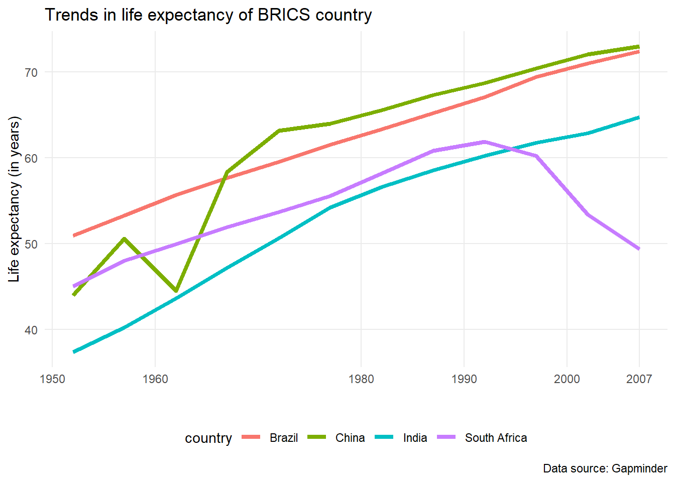
You can take it even further by creating a plot. You know that BRICS countries are Brazil, Russia, India, China and South Africa. You want to find trends in life expectancy. Note that there is no data for Russia
gapminder |>filter(country %in%c("Brazil", "Russia", "India", "China", "South Africa")) |>select(country, year, lifeExp) |>ggplot(aes(x = year, y = lifeExp, colour = country)) +geom_line(linewidth =1.5) +theme_minimal() +scale_x_continuous(breaks =c(1950, 1960, 1980, 1990, 2000, 2007)) +theme(legend.position ="bottom",panel.grid.minor =element_blank()) +labs(title ="Trends in life expectancy of BRICS country",x ="",y ="Life expectancy (in years)",caption ="Data source: Gapminder")
Wait a minute: why did south Africa’s life expectancy started to decline rapidly from the 1990s? One plausible reason would be the impact of HIV/AIDS and lack of antiretrovirals (ARVs). Welcome to data analysis.
You can see above the efficiency of the pipe operator. Think of the pipe operator as:
OR
We have introduced to the basics of data manipulation in R using the dplyr package in R. While we have covered a lot, the path is long. However, once you master these basic functions, you will not struggle in the following sections. These resources may be helpful: