── Attaching packages ─────────────────────────────────────── tidyverse 1.3.2 ──
✔ ggplot2 3.4.1     ✔ purrr   1.0.1
✔ tibble  3.1.8     ✔ dplyr   1.1.0
✔ tidyr   1.3.0     ✔ stringr 1.5.0
✔ readr   2.1.4     ✔ forcats 1.0.0
── Conflicts ────────────────────────────────────────── tidyverse_conflicts() ──
✖ dplyr::filter() masks stats::filter()
✖ dplyr::lag() masks stats::lag()5 Data Manipulation Part 2
Last week we introduced the basics of data manipulation using dplyr. This week I want u to continue to intermediate data manipulation in dplyr.
5.1 Renaming columns
You will notice that the column names in the gapminder dataset do not follow tidy principles. Naming things in a tidy we follow these principles:
No spaces between characters
all names should be in lower cases
only use underscore (_) to separate characters.
The tidyverse style guide. In our columns, the column names lifeExp are gdpPercap need to be renamed. We will use rename() function within dplyr:
then use rename() to change column names; we will save the new dataframe as gapminder_new
gapminder_new <- gapminder |>
  rename(life_expectancy = lifeExp,
         gdp_per_capita = gdpPercap)

head(gapminder_new)
# A tibble: 6 × 6
country continent year life_expectancy pop gdp_per_capita
<chr> <chr> <int> <dbl> <int> <dbl>
1 Afghanistan Asia 1952 28.8 8425333 779.
2 Afghanistan Asia 1957 30.3 9240934 821.
3 Afghanistan Asia 1962 32.0 10267083 853.
4 Afghanistan Asia 1967 34.0 11537966 836.
5 Afghanistan Asia 1972 36.1 13079460 740.
6 Afghanistan Asia 1977 38.4 14880372 786.The dataframe is updated with changed column names. However, when working with data with many columns, it would be time consuming to change each column. Fortunately, within the package janitor there is function called clean_names that change all the column names into a tidy way. Install the janitor package first:
After install it load it: and use the clean_names() function:
Attaching package: 'janitor'The following objects are masked from 'package:stats':
chisq.test, fisher.test# A tibble: 6 × 6
country continent year life_exp pop gdp_percap
<chr> <chr> <int> <dbl> <int> <dbl>
1 Afghanistan Asia 1952 28.8 8425333 779.
2 Afghanistan Asia 1957 30.3 9240934 821.
3 Afghanistan Asia 1962 32.0 10267083 853.
4 Afghanistan Asia 1967 34.0 11537966 836.
5 Afghanistan Asia 1972 36.1 13079460 740.
6 Afghanistan Asia 1977 38.4 14880372 786.See that untidy column names were changed automatically.
5.2 Converting column data types
Remember we discussed 3 data types:
character
numeric
logical
In a dataframe, you can find the data type of the column by using class() function
You can also use the str() to find the data types of all columns in the dataframe:
tibble [1,704 × 6] (S3: tbl_df/tbl/data.frame)
 $ country  : chr [1:1704] "Afghanistan" "Afghanistan" "Afghanistan" "Afghanistan" ...
 $ continent: chr [1:1704] "Asia" "Asia" "Asia" "Asia" ...
 $ year     : int [1:1704] 1952 1957 1962 1967 1972 1977 1982 1987 1992 1997 ...
 $ lifeExp  : num [1:1704] 28.8 30.3 32 34 36.1 ...
 $ pop      : int [1:1704] 8425333 9240934 10267083 11537966 13079460 14880372 12881816 13867957 16317921 22227415 ...
 $ gdpPercap: num [1:1704] 779 821 853 836 740 ...
Sometimes you may find that the all values in a column would be saved as character when they are supposed to be numeric. You can change them as using as.numeric() function. Let us simulate some fake data:
gender <- c("male", "female", "female", "male", "female")

age <- c("18", "30", "45", "21", "54")

example_df <- data.frame(gender, age)

example_df
gender age
1 male 18
2 female 30
3 female 45
4 male 21
5 female 54In the example_df dataframe, you can see that the age column has been stored as character, which doesn’t make any sense:
Convert this:
If you want to convert it back to character, you can use as.character() function:
chr [1:5] "18" "30" "45" "21" "54"The only time this will not work is when you try to convert a character column such as gender into numeric; try it. Experiment with converting various column type with the gapminder dataset.
5.2.1 Factors
There is another data type we have not discussed: factors or what may be called categorical data. Factors are like characters, except that they have integers that correspond to characters. In our example_df dataframe, we may want to make the column gender a factor, where 1 = male, 2 = female.
  gender age
1   male  18
2 female  30
3 female  45
4   male  21
5 female 54'data.frame': 5 obs. of 2 variables:
$ gender: Factor w/ 2 levels "male","female": 1 2 2 1 2
$ age : chr "18" "30" "45" "21" ...The gender column has been changed to factor, with 2 levels.
Let us try to change the continent column in the gapminder dataset, we will try the dplyr method:
gapminder <- gapminder |>
  mutate(continent_factor = factor(continent))

str(gapminder$continent_factor)
Factor w/ 5 levels "Africa","Americas",..: 3 3 3 3 3 3 3 3 3 3 ...Here we have used mutate() to create a new column named continent_factor that is a factor. It has 5 levels, you can check this using the levels() function:
Creating new columns instead of changing the existing one is important in some instances, especially when you want to compare the data.
The focrcats package within Tidyverse was specifically create for factors, you may want to visit it to learn more about factors.
5.3 Create a new categorical column from a numeric column
In many cases, we may want to create a new categorical column that takes the conditions from a numeric column. For example, example, in the following ages:
1-12 = child
13-17 = adolescent
18-34 = young adults
35-55 = adults
Over 55 = older adults
We can use the case_when() function within mutate() to create this column. Let us generate some fake data;
set.seed(45)
###simulate a character vector with a length of 50
gender <- sample(c("male", "female"), size = 50, replace = T, prob = c(.45, .55))


## simulate a numeric vector, with a length of 50, from ages 1 to 75
age <- sample(1:75, size = 50)

fake_df <- tibble(gender, age)

head(fake_df)
# A tibble: 6 × 2
gender age
<chr> <int>
1 male 18
2 female 11
3 female 55
4 female 62
5 female 67
6 female 27Then compute a new column:
fake_df <- fake_df |>
  mutate(age_group = case_when(
    age >= 1 & age <=12 ~ "child",
    age >= 13 & age <= 17 ~ "adolescent",
    age >= 18 & age <= 34 ~ "young adult",
    age >= 35 & age <= 55 ~ "adult",
    age > 55 ~ "older adult"
  ))

fake_df
# A tibble: 50 × 3
gender age age_group
<chr> <int> <chr>
1 male 18 young adult
2 female 11 child
3 female 55 adult
4 female 62 older adult
5 female 67 older adult
6 female 27 young adult
7 female 41 adult
8 male 6 child
9 female 10 child
10 female 51 adult
# ℹ 40 more rowsPlot the new column:
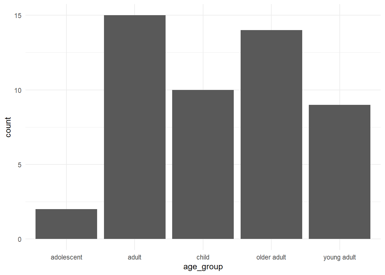
We have created a new column called age_group using the age column.
Experiment with the gapminder data. We may want to group countries according to their life expectancy based on the following rules:
if life expectancy of a country is lower than the world average, we will classify it as ‘low life expectancy’
if life expectancy of a country is higher than the world average, we will classify it as ‘high life expectancy’
We will only use observations from the year 2007:
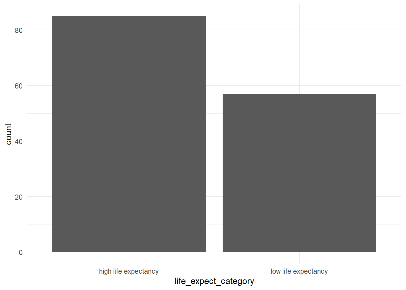
Create a new column:
We have created added a new column called life_expect_category; plot this column:
5.4 Missing data
Data rarely comes clean, and sometimes data can contain missing value. In R missing values are stored as NA. Once we go to the introduction to statistics section, we will deal with missing values.
5.5 Reshaping data
There are 2 types of dataframes: wide and long formats. I will use examples to illustrate both types.
Suppose we have data containing GDP increase rate of South Africa from 2010 to 2020 Let us create a long format of this dataframe:
year <- c(2010:2020)

gdp_rate <- c(2.8, 3.1, 3.3, 2.2, 1.9, 1.3, 1.5, 0.6, 0.8, 0.2, -7.0)

sa_gdp_long <- data.frame(year, gdp_rate)

sa_gdp_long
year gdp_rate
1 2010 2.8
2 2011 3.1
3 2012 3.3
4 2013 2.2
5 2014 1.9
6 2015 1.3
7 2016 1.5
8 2017 0.6
9 2018 0.8
10 2019 0.2
11 2020 -7.0The dataframe is in long format: We have one column reprenting all years, and gdp_rate column representing all values of GDP growth rate. What if we want to change to a wide format? We can use pivot_wider() function within tidyr package, also a part of tydiverse:
# A tibble: 1 × 11
  `2010` `2011` `2012` `2013` `2014` `2015` `2016` `2017` `2018` `2019` `2020`
   <dbl>  <dbl>  <dbl>  <dbl>  <dbl>  <dbl>  <dbl>  <dbl>  <dbl>  <dbl>  <dbl>
1    2.8    3.1    3.3    2.2    1.9    1.3    1.5    0.6    0.8    0.2     -7
You can see that in a wide format, each year is a column.
5.5.1 Excercise
In the gapminder data do the following:
Select country, year and life expectancy columns
filter rows rows from South Africa, Zimbabwe and Mozambique
reshape this data to a wide format
5.6 Joining data
You my have 2 dataframes with corresponding ID columns but with other different column names. Create a first dataframe:
country_name <- c("South Africa", "Zimbabwe", "Mozambique", "Botswana", "Eswatini", "Lesotho", "Namibia")

set.seed(187)
population <- sample(5000:15000, 7)

pop_df <- data.frame(country_name, population)

pop_df
country_name population
1 South Africa 7330
2 Zimbabwe 11323
3 Mozambique 7419
4 Botswana 9156
5 Eswatini 11783
6 Lesotho 14088
7 Namibia 8824Create a second dataframe:
country_name <- c("South Africa", "Zimbabwe", "Mozambique", "Botswana", "Eswatini", "Lesotho", "Namibia")

set.seed(50)
avg_age <- sample(23:35, 7)

age_df <- data.frame(country_name, avg_age)

age_df
country_name avg_age
1 South Africa 33
2 Zimbabwe 26
3 Mozambique 24
4 Botswana 29
5 Eswatini 25
6 Lesotho 30
7 Namibia 34Now we have 2 data frames: pop_df with a fake data on countries’ population and the age_df with a fake data on countries’ average age. The common name in both dataframes is country_name. We will use merge() function to join 2 dataframes:
  country_name population avg_age
1     Botswana       9156      29
2     Eswatini      11783      25
3      Lesotho      14088      30
4   Mozambique       7419      24
5      Namibia       8824      34
6 South Africa       7330      33
7     Zimbabwe      11323      26
Bingo!
There is more to joining data: merge() is a Base R funcion. There are other options of joining data using dplyr; see this guide